IMPaSTo: A Realistic, Interactive Model for Paint

William Baxter, Jeremy Wendt, and Ming C. Lin Department of Computer Science University of North Carolina at Chapel Hill {baxter,jwendt,lin}@cs.unc.edu http://gamma.cs. unc.edu/IMPaSTo/

Abstract

We present a paint model for use in interactive painting systems that captures a wide range of styles similar to oils or acrylics. The model includes both a numerical simulation to recreate the physical flow of paint and an optical model to mimic the paint appearance.

Our physical model for paint is based on a conservative advection scheme that simulates the basic dynamics of paint, augmented with heuristics that model the remaining key properties needed for painting. We allow one active wet layer, and an unlimited number of dry layers, with each layer being represented as a height-field.

We represent paintings in terms of paint pigments rather than RGB colors, allowing us to relight paintings under any full-spectrum illuminant. We also incorporate an interactive implementation of the Kubelka-Munk diffuse reflectance model, and use a novel eightcomponent color space for greater color accuracy.

We have integrated our paint model into a prototype painting system, with both our physical simulation and rendering algorithms running as fragment programs on the graphics hardware. The system demonstrates the model's effectiveness in rendering a variety of painting styles from semi-transparent glazes, to scumbling, to thick impasto.

CR Categories: 1.3.4 [Computing Methodologies]: Computer Graphics-Graphics Utilities; 1.3.7 [Computing Methodologies]:

Computer Graphics-Three-Dimensional Graphics and Realism

Keywords: Non-photorealistic rendering, Painting systems, Simulation of traditional graphical styles

1 Introduction

Each medium used in painting has particular characteristics. Viscous paint media, such as oil and acrylic, are popular among artists for their versatility and ability to capture a wide range of expressive styles. They can be applied thinly in even layers to achieve deep, lustrous finishes as in the work of Vermeer, or dabbed on thickly to achieve almost sculptural impasto effects, as in the works of Monet. With a scumbling technique, short choppy semi-opaque

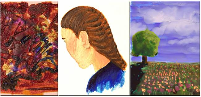
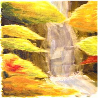
Figure 1: A painting hand-made using IMPaSTo, after a painting by Edvard Munch.

brush strokes create a veil-like haze over prevIous layers [Gair 1997].

It is a challenge to design an interactive model that captures the full range of physical behavior of such paint. Rather than attempt to simulate paint based on completely accurate physics, we aim instead to devise approximations which capture the high-order terms, and include heuristics which model the desired empirical behaviors not captured by the physical terms.

Paint is made by mixing finely ground pigments with a vehicle. Linseed oil is the vehicle typically used in oil paints, while in acrylics it is a polymer emulsion. Both of these are non-Newtonian fluids, and as such, are difficult to model mathematically. Basic properties of non-Newtonian fluids, like viscosity, change depending on factors like shear-rate¹• Furthermore, the key feature of interest in painting is how these fluids interact with the complex, rough surfaces of the canvas and brush, which means the mathematics must deal with geometrically complex moving boundary conditions and free surface effects. Finally, in addition to these challenges, a rough calculation shows the effective resolution of real paint is at least 250 DPI², and real paintings often measure many square feet in size.

Paint also features many stunning optical properties. The observed reflectance spectrum of a paint is due to a complex subsurface scat-

1The best-known example of this is ketchup, in which viscosity reduces under high shear rate, e.g., when shaken.

2Strokes often exhibit fine scale features on the order of the width of a single bristle. A typical hair is about 80 microns wide, which translates to a bare minimal resolution of at least 250 dots per inch (DPI), and probably 500 DPI or more to ensure an adequate Nyquist sampling rate.

tering and absorption phenomenon. The result is a richly non-linear behavior in the perceived color of paint depending upon both the thickness of a layer of paint and upon the mixture of pigments involved. Both of these nonlinearities are absent in the linear, additive RGBA color model typically used in computer graphics.

In addition to focusing on the plausible physical and optical behavior of paint, we also aim to provide an expressive vehicle for the users to interactively create original works using computer systems. This set of goals introduce strict constraints and challenges on the design and implementation of a computational model for an oil- or acrylic-like paint medium.

Main Contributions: In this paper, we present an interactive method for modeling paint media based on simplified physics and heuristics particularly tailored for use in real-time painting simulation. The three-dimensional paint surface is represented in "2.5D" using multiple height fields, with pigment concentrations and a volume (or height) stored at every pixel. The simulation is based on a conservative advection algorithm which preserves both overall paint volume and pigment mass even when the paint is spread thinly. The surface painted upon is also represented with a height field which the paint algorithm incorporates into its calculations to achieve realistic stroke texture over rough canvas or paper. We allow for one wet layer of paint at a time and an unlimited number of dry layers, which can be accumulated to create optical layering effects.

To more accurately model the non-linear chromatic behavior of real paint blending and layering, we have also implemented a color mixing and compo siting engine based on the Kubelka-Munk (K-M) model. Instead of accepting the limitations of RGB color space, we perform all color calculations in a custom eight-wavelength color space, which is dynamically determined at runtime to achieve best results for a particular full-spectrum lighting environment.

In order to achieve near real-time performance, both the paint transport and paint rendering are implemented in graphics hardware using programmable fragment shading capabilities. This approach allows for real-time interaction with the paint while calculating both the K-M reflectances and dynamic lighting of the paint surface on the fly, which would otherwise be difficult to achieve on a desktop PC.

We have incorporated the paint model into a prototype painting system, which demonstrates the capabilities of our paint medium. We measured the full-spectrum reflectances of several oil paints commonly found on an artist's palette and imported those into our system for users to paint with.

In order to manipulate the three-dimensional paint, our system provides users a three-dimensional brush which they control naturally using either a tilt-sensitive 5-DOF tablet or a full 6-DOF haptic armature. The user can build up layers and create paintings in a thick, impasto style, or use the paint more sparingly and with a reduced opacity to achieve thinner styles.

Since we store paintings in terms of pigments rather than colors, all pigments can be changed at any time to explore different possibilities, such as the effect of globally replacing one shade of green for another. The potential also exists for very accurate physical reproduction by using the recorded per-pixel pigment concentrations to create a hard-copy using real paint.

Organization: The rest of the paper is organized as follows. We provide a brief survey of related work in Sec. 2. We present an overview of the interactive painting system and the user interface in Sec. 3. We describe our method for modeling the physical behavior of paint in Sec. 4. In Sec. 5 we present our real-time implementation

of the Kubelka- Munk model. We discuss the implementation issues and demonstrate the results of our model in Sec. 6.

2 Previous Work

A number of researchers have investigated simulation and rendering of paint and other artistic media. We present a brief, though not exhaustive, summary of related work below.

2.1 Modeling Natural Media

Researchers have presented a wide variety of methods for simulating the physical properties of natural media, including charcoal, wax crayon, clay, watercolor, and other paints.

The most closely related works are those of [Baxter et al. 2001] and [Cockshott et al. 1992]. The former presents a naturalistic painting system using an efficient interactive model for thick paint, which is based on additive RGB blending. The latter presents a cellularautomata model for the relaxation behavior of liquid paint on a flat surface. The method seems to be interactive but it does not propose any approach for how a brush should interact with this paint model. The rendering used is a simple bump-mapping technique.

[Curtis et al. 1997] used a form of the shallow water and diffusion equations in their watercolor simulation with excellent results. However, their formulation is specific to thin, watery paint.

A number of researchers have generated convincing oriental-style ink painting systems, and some have developed sophisticated deformable brush models. See [Chu and Tai 2002] and [Saito and Nakajima 1999] for example. These systems are also for thin, water-color like paint, rather than thick oil-like paint. But some have incorporated canvas texture into their algorithms. The degree of interactivity varies, but Chu and Tai appear to have a very usable interactive system.

[Rudolf et al. 2003] simulate wax crayons, taking into account the height of the drawing surface.

Corel Painter ([Corel 2003]) is a commercial product that features a variety of digital natural media, though physical properties of the media are not simulated, just the appearance, apparently in RGB color space.

[Hertzmann 1998; Hertzmann 2001; Hertzmann 2002] present a number of automatic approaches to the generation of painterly renderings by heuristically placing and aligning strokes based on properties of an input image. The latter additionally uses a height field and bump-mapping to generate strokes with added dimension.

2.2 Kubelka-Munk

[Kubelka and Munk 1931; Kubelka 1948; Kubelka 1954] presented the Kubelka-Munk (K-M) equations to accurately approximate the diffuse reflectance of pigmented materials like paint given descriptions of their constituent pigments and pigment concentrations.

In computer graphics, [Hasse and Meyer 1992] demonstrated the utility of the K-M equations for rendering and color mixing in both interactive and offline applications, including a simple "airbrush" painting tool. [Dorsey and Hanrahan 1996] used K-M layer compositing to accurately model the appearance metallic patinas. [Curtis et al. 1997] also used the K-M equations for optically compositing thin glazes of paint in their watercolor simulation, and [Rudolf

Figure 2: The physical system setup with a tablet interface. We use the Wacom Intuos2 line of tablets which reports stylus X- Y tilt as well as pressure and X-Y location. From these 5 measurements we derive a 3D transform for the brush. We also support the Phantom haptic input device.

et al. 2003] used the same form in their wax crayon simulation. None of these implementations offers the real-time rendering desired for interactive applications.

3 Overview

In this section we give a brief overview of our painting system and its user interface design.

3.1 System Architecture

In order to test the effectiveness of our viscous paint model, we have created an enhanced interactive painting system based on our previous prototype called dAb [Baxter et al. 2001]. With the new paint model, IMPaSTo, we allow the user to choose between a tablet interface (Wacom Intuos2) or a haptic interface (Phantom), either of which serves as a physical metaphor for the virtual brush. Just as in dAb, the brush head is modeled with a spring-mass particle system skeleton and a subdivision surface. It deforms in response to contact with the virtual canvas. A wide selection of common brush types is made available to the artist. Fig. 2 shows the physical setup of our system with the tablet interface. A schematic diagram illustrating how various system components are related is shown in Fig. 3.

Our interface gives the user many of the digital advantages one would expect, such as the ability to undo and redo changes at the touch of a button, and to save and manage multiple revisions. In addition, the user can instantly dry paint, or keep paint wet as long as desired, and can change the paint opacity at any time even after finishing the painting.

4 Interactive Paint Simulation

With our dynamics algorithm, we wish to capture the general physical properties of paint interacting with a brush that are listed in

1. Paint moves in the direction pushed

2. Paint is conserved (neither created nor destroyed)

3. Brush-canvas paint transfer requires physical contact and is greater when the brush is moving.

4. The more paint is loaded on a brush, the more will be deposited on the canvas

5. The more paint is on the canvas the more will be picked up by the brush.

Table 1: The five general physical principles which govern our physical paint model.

Table 1.

A diagram of the steps in the algorithm we have developed is shown in Fig. 5. The algorithm basically consists of a conservative advection stage followed by carefully designed paint transfer rules. We describe each in detail below. Our paint model also allows for an unlimited number of layers of dry paint to be accumulated. We describe the algorithm for the drying process as well.

We represent the canvas as a 2D uniform grid with pigment concentrations and paint volume stored at each cell. The brush head is represented using a subdivision surface as in [Baxter et al. 2001]. We store the brush's paint attributes (per-cell pigment concentrations and per-cell paint volume) in a separate grid and map this grid onto the brush surface.

4.1 Paint Motion

Paint motion is driven and dominated by boundary conditions. On the one side is the paint's boundary with the moving brush, and on the other, the boundary with the stationary canvas. We simplify the actual physics of the situation by taking these boundary velocities to be the dominant terms, and deriving paint velocity in a straightforward manner from them. We concentrate our numerical effort in accurately moving, or advecting, paint according to the determined velocity field. First we will detail our advection scheme and then describe how we compute the velocity field.

4.1.1 Advection

The first two of the desired paint features listed in Table 1 are handled by our conservative advection algorithm, which is Stage 3 in the overall paint pipeline (Fig.5). Much research exists on conservative numerical solutions to hyperbolic partial differential equations. The standard text on the topic is [LeVeque 1992]. We present a basic variation of one such method here for solving the advection PDE.

Essentially we are given a scalar quantity q, such as the concentration of a pigment, and we wish to determine how that quantity evolves over time under a specified velocity field v. Mathematically, the problem can be expressed as finding the solution to the partial differential equation:

aq

at = -(v· \7)q.

(1)

In one dimension the problem reduces to just

aq aq

-=-v-

at ax'

(2)

·

~	l'orce Feedback		Voxclizcd Brush		1Jpdated
	(optional)		&		Pigment
			Brush Motion		Concentrations	Kubelka-Munk
		3D Brush		Paint
	q	Simulator	q	Simulation	q	Blending &	q
						Compo siting

Figure 3: System Architecture. We start with input from either a pressure- and tilt-sensitive tablet or Phantom haptic 10 device, then simulate the brush, simulate the paint, and render the painting's pigment concentrations into afinal RGB image for display. Fig. 5 details the 3D Paint Simulation stage further, and Fig. 6 shows the details of the K-M Rendering stage.

and if v is constant, the solution is just q(x, t) = q(x - vt,O), i.e. the initial quantities at time 0 are just translated by vt. Once we go to higher dimensions, the solution is not so simple, even for time-invariant velocity fields.

In a conservative numerical scheme for a hyperbolic conservation law, one constructs a flux function F that represents how much of the conserved quantity leaves and enters each cell of the computational grid. By ensuring the flux lost by one cell is always gained by another we can guarantee the method will be conservative. A numerical solution to the ID advection problem can be written in terms of flux as

n+l n 6t ( (n ) (n ))

qi = qi + 6x F qi-l/2 - F qi+l/2

The q values are stored at cell centers, and are interpreted as cell average values. The total amount of q in the cell initially is thus qi6x in ID or qi,j6x6y in 2D. The fluxes are computed at cell edges and represent the amount of material crossing that cell boundary, with positive fluxes denoting flow in the +x direction.

We diverge from the typical staggered grid formulation above and instead use a cell-centered grid, where both velocity and advected quantities are defined at the center of each cell. The numerical scheme we use is then as follows, explained first in ID for simplicity (see Fig. 4). Given a discrete velocity field Vi defined at cell centers, translate each column of q by vi6t. The total amount in cell i initially is qi6x, and an amount qilvi6tlleaves the cell under the velocity field, leaving qi(6x - IVi6tl) behind. Note that in order for cell i to not lose more flux than it originally possessed, we must have 6x - I Vi 16t > O. This imposes a limit on the maximum velocity possible, namely IVil < 6x/6t, commonly known as the CFL condition. Cell i may also gain flux from its neighbors. The amount gained from cell i-I is either 0, if Vi-l < 0, or qi-l Vi-l 6t otherwise. A similar expression exists for flux gained from cell i + 1.

The same basic scheme can be carried out in higher dimensions. For instance, in 2D, given a cell-centered velocity Vi,j = (u, v) we can treat the column of q as moving by u6t in the x direction and v 6t in the y direction and determine flux donated to other cells just as we did in the ID case.

In order to keep the computational requirements as low as possible, we use only 2D. To handle the third dimension, we treat the volume of paint in each cell as another scalar to be advected along with pigment concentrations. In other words we advect the height field according to the velocity we compute.

We have found one modification to the above algorithm to be useful. With the algorithm just as described above, it is quite possible to completely advect paint off of a particular canvas cell. This makes the canvas seem to be made of a material like Teflon. In order to

qi

qi

qi-l

Area=qiAx

Vi-l -

·

Vi-l -

Vi+l -

Vi+l -

i-l

i+l •••

i-l

i+l •••

(3)

Figure 4: ConsenJative advection flux computation in lD. Cell i + 1 gains a flux of qi I Vi I 6t from cell i, and cell i loses the same.

better model the adhesion and absorption of paint into the canvas surface, we simply do not allow advection to remove all the paint in a cell. The computed flux quantity is clamped to leave at least a parameter-defined minimum quantity behind.

4.1.2 Computing Velocity

The preceding description of our advection calculation was predicated on the a priori knowledge of a velocity field to use. In real painting this velocity field comes from a number of sources. As mentioned, the main source is the frictional forces imposed by the brush on the one side of a layer of paint, and by the stationary canvas on the other. Any viscid fluid will have zero slip (tangential) velocity at the interface between the fluid and a solid boundary. So during a paint stroke, within the thin layer of paint trapped underneath the brush, the paint in contact with the brush has the brush's velocity, while paint in contact with the canvas has the canvas's velocity. Since paint is a continuum, all possible velocities between zero and the brush speed must exist within the layer of paint. Thus as a first approximation, a reasonable 2D velocity to assign the paint is 1/2 of the of the brush's tangential velocity relative to the canvas surface. This kinematic brush velocity, Vb, is the first component of the total velocity used. This velocity only applies to cells in the canvas surface which are in contact with the brush as determined in Stage 1 of the computation pipeline (Fig. 5).

But paint is not just two-dimensional, and although painting a stroke is primarily a motion in the 2D canvas plane, the out-of-plane motion and vertical force of the brush are also important. Paint is an incompressible fluid and it is affected by internal pressure forces. For instance, when a force is applied downward from above, the pressure field that develops internal to the paint induces a flow in the direction of the negative pressure gradient. In other words it causes

	Stage 1		Stage 2		Stage 3		Stage 4		Stage 5
Q	Compute	Q	Compute	Q	Advect	Q	Deposit	Q	Pick up
	Penetration		Cell Brush		Volume and		Volume and		Volume and
	Mask		Velocity		Pigment		Pigment		Pigment
		~ If early exit (Occlusion query) )

Figure 5: Steps in 3D Paint Simulation. Each of the above boxes is implemented using one or two fragment programs on the GPu. After computing the penetrations we use the occlusion query to determine if any canvas fragments were in contact with the brush, and exit early if not.

the paint to flow outward in any unconstrained direction. To model this "squishing" behavior we use a simple heuristic. First, for every cell in the 2D paint grid where the brush penetrates the heightfield surface, we compute the amount of penetration, p (done in the first stage, Fig. 5). Next we compute the 2D gradient of the penetration amount, \7 p, and define a heuristic "pressure" -driven velocity to be a constant times that value, v_p = -c\7p. This pressure driven velocity, v_p is then simply added onto to the brush velocity Vb to get the total velocity at each cell of brush-canvas contact. Note that this can be seen as an approximation of the pressure term on the right hand side of the full Navier-Stokes equations for fluid motion:

av 2

at = -(v· \7)v + v\7 v - \7p + F, \7. v = 0 (4)

where we substitute amount of penetration for the amount of internal pressure, assuming the two to be roughly proportional.

When laying down a stroke, we move the brush along the stroke path no more than one cell width at a time to ensure that Vb does not violate the CFL condition. Also, after adding in v_p, we clamp the final x and y velocity components to be within [-1,1], just in case v_p is unusually large.

4.2 Paint Transfer

The paint transfer algorithm is responsible for determining how much paint moves from the brush to the canvas and vice versa. Each of the remaining desiderata in Table 1 is handled via our transfer algorithm (Fig.5, Stages 4 and 5).

The first assumption we make is that at any given cell where brushcanvas contact is occurring, the transfer flow is uni-directional. That is to say, if paint is being deposited onto the canvas at a particular cell, it cannot also be loading into the brush simultaneously. Note that since this is a per-cell determination, it is still possible that at any given instant some parts of the brush are loading paint, while others are depositing paint. The direction of the flow is determined by whether there is more paint on the canvas, a_c, or more paint on the brush, ab. Rather than the full amount of paint in the canvas cell, we define a_c to be the full volume times the fraction by which the brush is determined to be penetrating the paint surface in Stage l(Fig. 5). In this way, one can still deposit paint on the surface of a thickly covered canvas by brushing lightly.

Algorithm 1 gives the full calculation used. First, no paint is transferred if the brush is not in contact. Then, the direction of flow is determined by whether ab or a_c is greater, and the base amount of flow is computed as a fraction of either a_c or ab depending upon the direction. The base transfer amount is then modified in several important ways. The transfer is gently cut off to zero when a_c is nearly equal to ab to prevent developing unstable oscillations of the

paint transfer back and forth. Next we cut off the transfer amount gradually if the brush velocity is below a threshold to account for the need for some sliding friction to "pull" paint out of the brush. Without this, the brush appears to ooze paint unnaturally. Finally, the transfer amount is clamped to a maximum value to make the paint transfer more even. The pseudocode shows all of these steps and includes parameter values we have found to work well. To put the constants in context, our paint thickness for a thin painting is typically around 0.001 units and around 0.1 for a thicker style. Velocity is in terms of cells per timestep, so 1.0 is the maximum possible velocity component.

(Xbc, Xcb) f- COMPUTEBRUSHTRANSFERAMouNT(a_c, ab, v) [> let a_c be amount of paint penetrated in canvas cell

[> let ab be amount of paint on corresponding brush cell [> let v be tangential velocity of brush

[> let Xbc be the amount transferred from brush to canvas [> let Xcb be the amount transferred from canvas to brush [> let XFER_FRACTION = 0.1

[> let MAX_XFER_QUANTITY = 0.001 [> let EQUALPAINT-CUTOFF = 1/30 paintDiff f- ab - a_c equalPaintCuto f f f-

c1amp(lpaintDif fl/EQUALPAINT _CUTOFF, 0, 1) velocityCutof f f- smoothstep(0.2, 0.3, Ilvll)

xferDir f- sign(paintDiff)

ifxferDir> 0

then amt f- ab else amt f- a_c end

amt f- amt * XFER_FRACTION

amt f- amt * equalPaintCuto f f * velocityCuto f f amt f- c1amp(amt, 0, MAX_XFER_QUANTITY) ifxferDir> 0

then (Xbc, Xcb) f- (amt,O) else (Xbc, Xcb) f- (0, amt) end

ALGORITHM 1: The paint transfer algorithm

When paint is transferred either direction, or is moved by the advection algorithm, we compute the new pigment concentrations on the affected brush or canvas cells by a simple volume-weighted average.

4.3 Paint Drying

Our paint model supports the drying of wet paint in order to allow the user to build up paintings out of many layers of paint. The process we support is different from the drying of actual paint in that

Texture

Use

base canvas reflectance		R
painting reflectance (temporary)		R
painting RGB composite		R
painting pigment concentrations	I	R
painting thickness/paint volume (base/dry/wet)	I	R
brush penetration on canvas (base/dry/wet)	I
brush velocity (x,y,z)	I
brush pigment concentrations	I	R
brush RGB composite		R
brush paint volume	I	R
paint undo buffer	I

Table 2: Textures used in GPU implementation. '[' indicates use in paint interaction and dynamics; 'R' indicates the texture is used in rendering.

wet paint is always completely wet, and dry paint is completely drl. However, these are the two extremes which are typically desired. Given a layer of wet paint we allow fractional drying of that layer as a percentage of the overall thickness. So if the user elects to dry the paint by 25 percent, we will create a new dry layer out of the bottom quarter of the wet layer, leaving 3/4 of the wet paint in tact.

While the memory and processing requirements to support an unlimited number of wet layers of paint would be prohibitive, it is possible for us to support as many dry layers as virtual memory will hold, since they are static, and for the purposes of painting a stroke, can be treated the same as we treat the static base canvas texture. Thus we only need to know their combined thickness, which can be computed just once. We also need to maintain the combined reflectance of all the dry layers for use by the rendering algorithm, which will be discussed in detail in the next section.

When a new layer is dried, the combined thickness and reflectance information is just a function of the current composite thickness and reflectance and the thickness and pigment concentrations of the new dry layer. The computation involved in updating the reflectance will be discussed in more detail in the next section, and is the same process described in Fig. 6. Note that even though the runtime system does not need the dry layer's pigment information once a drying operation is complete, we must keep that data nonetheless for use when changing the lighting spectrum.

4.4 GPU Implementation

We have implemented our paint transfer algorithm using an NVIDIA GPu. All of the relevant data is stored in textures and operated on by fragment programs. Table 2 lists all of the textures used, with the exception of temporaries for holding intermediate results. In this implementation one canvas or brush cell is represented by a single texel of a texture. We have used half-precision floating point for all of the textures, except some of the small intermediate textures required in computing the rendering. In our GPU implementation, each of the stages in Fig 5 is performed by one or two fragment programs.

One aspect of the problem is worth pointing out. Whether implementing on GPU or CPU, one key implicit requirement of the algorithm is to establish a mapping between brush texel space and canvas texel space. On the GPU, we do this simply by rasterizing the textured brush head mesh under orthographic projection into one of

3Technically, oil paint does not dry, but rather oxidizes.

the canvas textures via the Render-to-Texture extension. The texture coordinates input into each fragment are in brush texture space, and the raster window coordinates give the corresponding location in canvas space. This is how we perform updates to the canvas textures. To update the brush textures we essentially want to use canvas space textures to texture the brush mesh. This can be accomplished by switching the roles of the brush texture coordinates and 2D projected brush vertices, and rendering the result into one of the brush textures. (A simple scale and translate of the values is required, and these are easily incorporated by pushing an extra transform on the model and texture matrix stacks of the GPU). With this setup, the raster window position gives the brush texture space coordinate of each fragment, and input texture coordinates (i.e. projected brush vertex locations) give the corresponding canvas texture coordinate.

As can be seen, computing the brush to canvas mapping really is a rasterization problem, making this part of the problem an ideal fit for the GPu. To implement on the CPU one would essentially have to write a software rasterizer. The rest of the algorithm also maps well to the GPU since we have formulated all of the operations (e.g. gradient and advected flux) locally so that they depend at most on their immediate neighbor fragments.

Another detail worth mentioning is the tiling implementation. Most image manipulation programs use some form of tiling to speed up operations. For undo as well as for rendering computations, we break the painting up into tiles of size 64 x 64. When a brush stroke is about to modify the data in a tile, the original data must be backed up somewhere to provide the ability to undo the action. In our previous CPU-based painting system this undo information was stored in system memory, but for a GPU-based implementation, copying to system memory introduces an unacceptable penalty due to the slow read-back from the GPU memory. Instead we allocate one additional "undo texture" in the graphics card memory and dynamically allocate undo tiles out of it. We are thereby able to use fast texture-to-texture copies on the GPU to save the necessary undo data for each tile. The use of tiling also speeds up the rendering computation tremendously, because only dirty (that is, modified) tiles need to be updated.

5 Paint Rendering

In this section we describe how we render our simulated paint using measurements of real paint samples as source data and the well-known Kubelka-Munk pigment mixing and layer compo siting equations.

5.1 Color Space Representation

As mentioned in Section 2, the Kubelka-Munk (K-M) model has been used previously in order to render pigmented materials that exhibit subsurface scattering and absorption. Although both [Curtis et al. 1997] and [Rudolf et al. 2003] use K-M to simulate artistic media, they both used simpler rendering during user interaction, and then added the more accurate colors as a post processing step. [Hasse and Meyer 1992] used a custom four-wavelength representation of the K-M parameters based on Meyer's previous work [Meyer 1988], while the others worked in standard threewavelength RGB space.

Meyer's four-wavelength color encoding was developed to be both more accurate than RGB and still efficient enough for computer graphics, circa 1988 [Meyer 1988]. This encoding was based on integrating against the human visual response functions in ACC color

·

Stage 1		Stage 2	Stage 3		Stage 4
Calculate	Q	Compute	Q	Q		Q
Pigment Mix		Reflectance &			Convert
		Transmittance			toRGB
(K/Smix)		(R & T)
				tr
	(If not last layer)

Figure 6: Steps in Kubelka-Munk Rendering. We begin with per-layer pigment concentrations and volume (per-pixel thickness). Stage 1 computes the absorption and scattering coefficients (K / Smix) for a layer of paint using Eq. 5, then Stage 2 uses this to compute the reflectance and transmittance of that layer, according to Eqs. 7-9. Stage 3 uses Eq. 10 to composite the single layer's reflectance with the reflectance of all layers beneath it. We repeat Stages 1-3 for each layer from bottom to top, and finally in Stage 4 we convert the result to RGB according to the current light spectrum and other lighting parameters.

space. He used Gaussian quadrature in order to find four abscissae wavelengths that when integrated against, would improve modeling results compared to standard RGB models. However, Johnson and Fairchild point out that under some lighting conditions, ACC gives incorrect results. They suggest using full-spectral color representations and present a real-time full-spectral rendering environment [Johnson and Fairchild 1999].

In order for artistic media to be properly simulated, colors must blend properly. However, artists must also see the results of their actions continuously in order to react to the new output and produce painterly works. Also, it is useful for the artist to be able to preview how colors will appear under different types of lighting. In order to satisfy all of these conditions, we use a novel approach that combines Meyer's use of Gaussian quadrature, Johnson's use of full spectral data, and Kubelka- Munk color mixing.

5.2 Measuring the paints

In order to gain a true representation of paint media, we chose several standard oil paint colors that are common to an artist's palette (See [Gair 1997], e.g.). In order to measure these paints, we created thick, flat samples of each paint and mixtures of the paints in measured ratios. We then measured our samples' reflectances using Photo Research's Spectra Scan PR-715, a spectra-radiometer. In this manner we obtained 101 reflectance values for each sample in the visible spectrum (380-780nm). Our measurement rig was set up as in Figure 7 with the light source at approximately a 60degree angle from the sample's normal. The angle was chosen first to minimize the amount of specular reflection measured, and, second, because this geometry is significant in that the assumptions of K-M theory are only exactly satisfied for incident radiance that is either uniform and isotropic or in parallel rays at a 60 degree angle [Kubelka 1948]. We used a reflectance standard made of Fluorilon FW in order to measure the output of the light.

-26=

Figure 7: Our setup for measuring paint reflectances. Each paint was placed in turn at the sample location. Several measurements were made per paint sample and averaged.

5.3 Converting to Kubelka-Munk

After factoring out the light's energy spectrum from our sample measurements, we calculated the K-M absorption and scattering (K and S) coefficients for each paint sample at each wavelength. Given mixtures 1 < i < M of the pure pigments 1 < j < N, we use the following equation from K-M theory [Kubelka 1954; Hasse and Meyer 1992]:

Lj KjCij Lj SjCij

(5)

(1 - Roo,i)2 2Roo,i

This relates the reflectance of mixture i, Roo,i, to the absorption and scattering values of each constituent pigment, Kj and Sj, and their relative concentrations, Cij. Pigments not involved in a particular mixture are assigned zero concentration.

From Eq. 5 we can assemble a linear system (for each wavelength) of the form

(6)

where C = {Cij} is an MxN matrix containing the paint concentrations, and QR is an M x M diagonal matrix, containing the right-hand sides ofEq. 5 along the diagonal. The unknowns, K and S, are both N x 1 vectors.

In general, for M > 2N, the zero vector is the only solution, since the equations will have zero nullity (full column rank). So we seek instead a least-squares solution that minimizes AT A, subject to a constraint that enforces non-triviality of the solution. We can enforce this with a simple equality constraint on one of the variables, say Sk = 1 for some k. We further require that each Kj and Sj be positive. Together these requirements specify a simple quadratic program (QP) which can be solved using a standard QP solver. We made M = 71 measurements of different mixtures involving N = 11 different paints, including the N measurements of the pure pigments alone. We chose to enforce Sk = 1 for k corresponding to Titanium White. Note that regardless of how the equations are solved, it is always necessary to choose some value arbitrarily, since K and S always appear in ratio. Figure 8 shows the measured reflectances, computed K and S values, and reflectance computed from those K and S values for three of our paint samples, calculated as just described.

5.4 Lights, Sampling and Gaussian Quadrature

We wish to treat color as accurately as possible, but it is not feasible to store our full 100-wavelength K and S samples on a per-pixel

Pigment Reflectances

- Cobalt Blue

_ Alizarin Crimson

0.35 - Yellow Ochre

- Cobalt Blue

_ Alizarin Crimson

- Yellow Ochre

Kubelka-Munk K Values

0.8

0.4

12

·

Kubelka-Munk S Values

·

·

10

0.3

S 0.25

" "

§ 0.2

t)

"

~ 0.15

0::

0.1

~o 4~ ~o 5~ wo 6~ roo 7~ Wavelengths (nm)

0.7

~ 0.6 'S

~ 05 e. .5⁰.⁴

~

8 0.3 Vl

VJ 0.2

0.1

400 450 500 550 600 650 700 750

Wavelengths (nm)

400 450 500 550 600 650 700 750

Wavelengths (nm)

Figure 8: Some results from measuring real oil paints. The left graph shows the measured reflectances after factoring out the spectrum of the incident light source (dotted lines), and our computed reflectances after solving for K and S values (solid lines). The right two graphs show the Kublelka-Munk absorption (K) and scattering (S) coefficients computedfrom the measured reflectance data.

basis or to compute the K-M model per-pixel on all of this data in an interactive system.

Figure 9: A comparison of the same painting created in IMPaSTo under two different light sources. On the left, the painting is illuminated by a 5600K bulb. On the right, it is illuminated under CIE Fluorescent Illuminant F8. Graphs of the light spectra are in blue, the 8 sample wavelengths chosen by IMPaSTo in red, and the CIE XYZ integrating functions are shown in black for reference.

We thus turn to numerical integration for a way to reduce the amount of wavelength data we must use in per-pixel calculations. Fortunately, most naturally-occurring reflectance spectra, including those of common paint pigments, are fairly smooth functions, and are thus well approximated by polynomials of moderate degree. We take advantage of this by using a Gaussian quadrature numerical integration scheme [Warnick 2001] to compute the final conversion of per-wavelength K-M diffuse reflectances to RGB for display.

Our system stores the original 101 K and S samples for all paints, energy spectra for the lights, and base reflectances for the canvas and palette. Upon choosing one specific light spectrum (e.g., the CIE Standard Illuminant D65), an automated Gaussian quadrature engine finds eight sample wavelengths and weights using a weighting function based on the XYZ integrating functions combined with the light's energy spectrum (See [Foley et al. 1995] for more information on converting spectra to XYZ space). Then, we sample each of our complete spectra at the chosen wavelengths (See Fig. 9). We

chose to use eight wavelengths because it is a good fit with graphics hardware, enabling us to store the eight samples in either two textures or in one floating point texture packed as half-precision floating point.

Since our weighting function is guaranteed to be nonnegative, Gaussian quadrature will return sample wavelengths and weights internal to our integrating region. In this way, we choose the wavelengths that are influential to both our final integration function (based on the human visual system) and the lighting environment. For instance, if a bluish light is selected to illuminate the canvas, the system will choose eight wavelengths that are biased more toward the blue end of the spectrum.

5.5 Rendering Pipeline and GPU Implementation

We use fragment shaders written in NVIDIA's Cg programming language to calculate the overall RGB reflectance of the painted canvas, the palette and the brush bristles. As shown in Table 2, we use two textures that, with their eight channels, represent the concentrations of the eight pigments simultaneously allowed at any pixel, and then another texture as the thickness for the paint on that texel in that layer.

We use a multi-pass approach that allows for several layers of pigment to be stacked on top of each other. Our rendering pipeline closely follows the stages of Figure 6. Each stage is implemented as a separate fragment program. The first three fragment programs calculate the final reflectance of anyone layer of paint. Stage 1 calculates K j Sand S for the pixel by using Eq. 5, which maps nicely to graphics hardware (dot products and 4 channel adding). Stage 2 calculates the reflectance and transmittance for this one layer using the following:

b

V(KjS) (KjS + 2) 1

1 + KjS + btanh(bSd) bR sinh(bSd).

(9)

R

(7) (8)

T

Where d represents the thickness of one layer of paint. Stage 3 calculates the reflectance of this layer compo sited on top of the pre-

·

Scanned Paint

3 Samples 3 Samples

RGB wi K-M RGB Linear

Figure 10: The left column shows graded mixtures of Yellow Ochre and Prussian Blue under a 5600K light. The right four columns show computer simulations of the mixtures using different numbers of sample wavelengths and differing techniques. As can be seen, linear RGB blending wrongly predicts brown. Although our implementation of K-M blending does not match the scanned colors exactly, the important feature to note is that the result of using our 8-sample Gaussian quadrature is almost identical to that using 101 samples. Thus, given more accurate reflectance data as initial input, we should be able to match the real samples very closely.

vious layers using

T² R_prev

Rtot = R+ RR

1 - "prev

(10)

These three stages use the eight wavelengths chosen via Gaussian quadrature, and are iterated over once for each layer of pigment. In our implementation, only the wet paint is represented as pigments in the runtime data, requiring these multi-pass iterations. As paint dries, its reflectance is calculated and added into the base canvas. To change the light spectrum when dry layers are present, we do as many passes as are necessary in order to "bake" the dry paints into the base canvas' reflectance, and then need only perform these calculations once for the wet paints. Stage 4 uses our weights derived via Gaussian quadrature and the XYZ integrating functions in order to transform these 8 wavelength values into RGB space for display. Since the K-M calculations only give us the diffuse reflectance, we complete the lighting computation with per-pixel dot-product bump-mapping and Blinn-Phong specular highlights.

5.6 Color Comparison

Figure 10 shows the results of our rendering algorithm and comparisons of the blending results for our method and a number of alternatives. Note that we achieve nearly the same results with our 8-wavelength Gaussian quadrature as are obtained using all 101 wavelength samples, at greatly reduced runtime computational cost. Also note that the results when using fewer samples, as previous researchers have, are noticeably different.

Figure 11: A painting created with 1MPaSTo, after a painting by Vincent Van Gogh.

6 Results

We have tested our viscous paint model implementation on a 2.5GHz Pentium IV machine with an NVIDIA GeForceFX 5900 Ultra graphics card. Note that the CPU speed is not critical for interactive response, and IMPaSTo has also been used successfully on CPUs of less than IGHz. The time required to draw a stroke is almost completely dominated by the physical paint model, since the cost of the optical model is greatly reduced by our tiling and lazy evaluation. For a brush footprint of approximately 26x26, our paint simulation pipeline shown in Fig. 5 is able to run about 116 times per second, processing an average of 77,000 canvas cells per second (i.e. texels/sec). For a larger brush footprint of about 88 X 88, we can run the pipeline only 68 times per second, but texel throughput increases to 519,810 canvas cells per second. At these speeds we are able to keep up with the user for strokes of moderate speed. For faster strokes the input data is buffered and the stroke lags slightly behind the user. The improved texel throughput for bigger brushes is a strong indication that much of our time is spent in per-pass setup overhead and GPU context switches.

We have integrated our paint model with a prototype painting system to simulate an oil-like painting medium. We provide the user with a large canvas, then run the fragment programs only in the bounding rectangle of the region of brush contact. For the rendering we mark the canvas tiles through which a stroke passes as dirty and recompute reflectances and relight the canvas on a tile-by-tile basis as needed each time through the main display loop.

Fig. 12 shows examples of various styles, effects and paint textures that our paint model is capable of creating. These and other paintings shown in Figs. 11-18 demonstrate the range of paint-like effects our model achieves. Most of these paintings were created by amateur artists within a couple of hours, without much training or elaborate instruction. The footage in the supplementary video demonstrates the interactive performance and behavior of our model. The video is available at http://gamma.cs. unc.edu/lMPaSTo.

7 Summary and Conclusion

In this paper, we presented an interactive paint model for the oilor acrylic-like paints used most commonly in fine art painting. The main characteristics of our paint model include:

Figure 12: Our paint model is capable of expressing diverse styles and effects. Here are some examples created by our paint model: (a) thick painting strokes in an abstract painting; (b) thick strokes enhancing a figural painting, as well as thinner strokes that reveal canvas texture, and (c) a thinner glaze-like painting style. Note also the variety of styles represented in Figs. 11, and 13-18.

· An interactive paint model that captures the dynamic behavior of thick paint;

· A conservative, paint-volume preserving advection scheme, and realistic brush-canvas paint transfer heuristics;

· Real-time color pigment mixing and compositing based on the diffuse reflectance model described by Kubelka and Munk;

· Full-spectrum color calculations for accurate Kubelka-Munk mixing and prediction of real-world coloring under different lights.

• GPU implementation of both paint dynamics and rendering.

7.1 Limitations

There are currently a number of limitations to our approach. First the resolution we are able to achieve is limited due to computational costs, but we believe that a number of speed-ups to our GPU implementation can still be made, and at the same time GPU performance continues to increase as well.

While our technique for solving for K and S values using quadratic programming seems fairly robust and efficient, it minimizes error in K-S space, which does not necessarily give an accurate measure of perceptual error. Slightly better results might be obtained by solving a fully non-linear program in terms of least-squares error in the perceptually uniform L*a*b color space. An advantage of the QP formulation, however, is its convexity, which guarantees that any minimum is the global minimum.

It must also be said that the Kubelka-Munk equations are an idealization and do not simulate real light transport exactly. All of the caveats with Kubelka-Munk listed by [Curtis et al. 1997] apply to our work as well.

7.2 Future Work

In the future, we are interested in the capture problem of converting existing RGB or real-world image sources into our pigment-based representation. Another area of interest is methods for efficiently representing and manipulating the finer scale details, those on the order of single bristle widths. Finally, an area related to the last is better brush models that contain detail on that scale, and which react more naturally.

Since the Kubelka-Munk model is essentially a ID subsurface scattering model, there are some potentially interesting questions that remain unanswered regarding the connections between KubelkaMunk and other more recent subsurface scattering approximations such as BSSRDF, spherical harmonics and precomputed radiance transfer (PRT). We are interested in investigating these as well.

8 Acknowledgments

This paper was funded in part by Intel Corporation, the National Science Foundation, the NVIDIA Fellowship Program, the Office of Naval Research, and the U.S. Army Research Office. We would also like to thank the painters who used our system: Eriko Baxter, John Holloway, Andrea Mantler, and Heather Wendt.

References

BAXTER, W. v., SCHEIB, v., AND UN, M. C. 2001. DAB: Interactive haptic painting with 3d virtual brushes. In S1GGRAPH 2001, Computer Graphics Proceedings, ACM Press / ACM SIGGRAPH, E. Fiume, Ed., 461-468.

CHU, N. S., AND TAl, C. L. 2002. An efficient brush model for physically-based 3d painting. Proc. of Pacific Graphics (Oct).

Figure 13: A painting created with IMPaSTo.

Figure 14: A painting created with IMPaSTo.

Figure 15: A painting created with IMPaSTo.

Figure 16: A painting created with IMPaSTo.

Figure 17: A painting created with IMPaSTo.

Figure 18: A painting created with IMPaSTo.

COCKSHOTT, T., PATTERSON, J., AND ENGLAND, D. 1992.

Modelling the texture of paint. Computer Graphics Forum (Eurographics'92 Proc.) II, 3, C217-C226.

COREL. 2003. Painter 8. http://www.corel.comlpainter/.

CURTIS, C. J., ANDERSON, S. E., SEIMS, J. E., FLEISCHER, K. W., AND SALESIN, D. H. 1997. Computer-generated watercolor. In Proceedings of the 24th annual conference on Computer graphics and interactive techniques, ACM Press/AddisonWesley Publishing Co., 421-430.

DORSEY, J., AND HANRAHAN, P. 1996. Modeling and rendering of metallic patinas. In SIGGRAPH 96 Conference Proceedings, Addison Wesley, H. Rushmeier, Ed., Annual Conference Series, ACM SIGGRAPH, 387-396. held in New Orleans, Louisiana, 04-09 August 1996.

FOLEY, J. D., VAN DAM, A., FEINER, S. K., AND HUGHES, J. F. 1995. Computer Graphics: Principles and Practice. AddisonWesley Publishing Company.

GAIR, A. 1997. The Beginner's Guide, Oil Painting. New Holland Publishers.

HASSE, C. S., AND MEYER, G. W. 1992. Modeling pigmented materials for realistic image synthesis. ACM Trans. on Graphics I 1,4, p.305.

HERTZMANN, A. 1998. Painterly rendering with curved brush strokes of multiple sizes. Proc. of ACM SIGGRAPH, 453-460.

HERTZMANN, A. 2001. Paint by relaxation. Proc. Computer Graphics International, 47-54.

HERTZMANN, A. 2002. Fast paint texture. NPAR 2002: ACM Symposium on Non-Photorealistic Animation and Rendering, 91-96.

JOHNSON, G. M., AND FAIRCHILD, M. D. 1999. Full-spectral color calculations in realistic image synthesis. IEEE Computer Graphics & Applications 19, 4.

KUBELKA, P., AND MUNK, F. 1931. Ein beitrag zur optik der farbanstriche. Z. tech Physik 12, 593.

KUBELKA, P. 1948. New contributions to the optics of intensely light-scattering material, part i. J. Optical Society 38, 448.

KUBELKA, P. 1954. New contributions to the optics of intensely light-scattering material, part ii: Non-homogenous layers. J. Optical Society 44, p.330.

LEVEQUE, R. J. 1992. Numerical Methods for ConsenJation Laws. Birkhauser Verlag.

MEYER, G. W. 1988. Wavelength selection for synthetic image generation. CVGIP4I, 57-79.

RUDOLF, D., MOULD, D., AND NEUFELD, E. 2003. Simulating wax crayons. In Proc. of Pacifc Graphics, 163-172.

SAITO, S., AND NAKAJIMA, M. 1999. 3d physically based brush model for painting. SIGGRAPH99 Conference Abstracts and Applications, 226.

WARNICK, K. F. 2001. Gaussian quadra-

ture and iterative linear system solution methods. http://www.ee.byu.edu/ ee/class/ee563/notes/gq _tutorial.pdf".

WYSZECKI, G., AND STILE, M. 1982. Color Science. Wiley.