No embedded latex yet.
I started with the graph y=f(x) of f in the x,y-plane and the geometric approach for ẋ=f(x).
Note that I plotted a wrong solution in the t,x plane on the right. Explain!
Anti-derivatives F of 1/f on intervals between zero's provide all solutions via F(x)=t+C.
In each such interval take your pick of x0 to define such F by F(x)=∫ x0x 1/f.
I would pick x0 where |f(x)| is maximal.
Use yf(x)=1 ro relate finite time blow up to bounded areas between that graph and the x-axis.
Use improper integrals to explain.
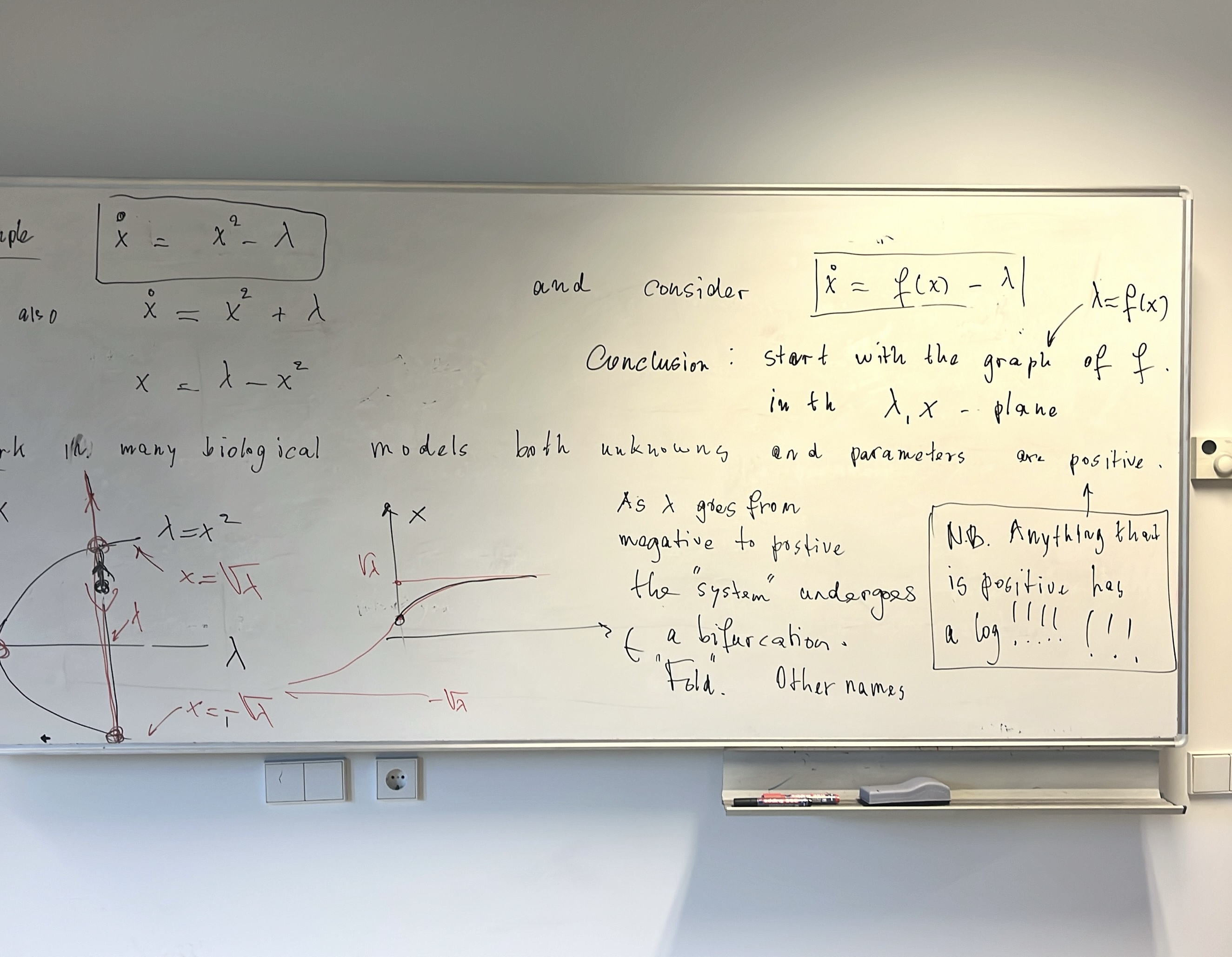
I replaced y by λ in the graph of for the study of ẋ=f(x)-λ.
We also considered ẋ=f(x)-λx for a specific case of f.
Compare ẋ=x(1-x) -λx to ẋ=x(1-x) -λ in the context of fishing quota.
Divide ẋ=x(1-x) -λx by x to introduce ln x as a new independent variable?