Section 2.1
The first example of \(\dot x=f(x)\) is \(\dot x=\sin(x)\). It returns in Section 4.1 as \(\dot\theta=\sin(\theta)\).

Strogatz does not introduce the anti-derivative \(F\) defined by \[F=\ln(\frac{1-\cos}{\sin})\,\quad F'=\frac1f=\frac1\sin,\quad F(0)=\frac\pi2\] and talks about headaches instead.

Too bad. This \(F\) immediately gives all solutions \(x(t)\) which lie between the steady states \(x=0\) and \(x=\pi\) in the implicit form \[F(x)=t+C.\] Figure 2.1.1 is on the board below. For the other ranges that you see from the global analysis you maybe have to think a bit.

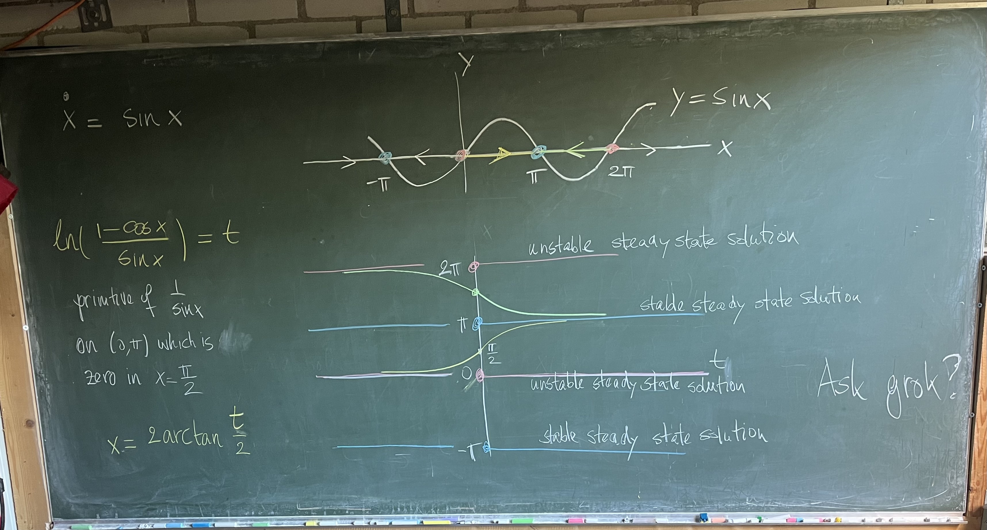
Figure 2.1.3 strangely omits negative \(t\). The above global picture is missing and \(F\) is not even mentioned.

Some clumsy form of \(F(x)\) with csc and cot leads to a rant about an even clumsier formula for the solution with \(x(0)=x_0\).

The formula \[ F(x)=t+F(x_0) \] is missing in action.

Section 2.4
For the stability analysis of a steady state \(x^*\) of \(\dot x=f(x)\) Strogatz writes \[x(t)=x^*+\eta(t)\] to obtain \[\dot\eta=f(x^*+\eta)\] for \(\eta=\eta(t)\).

Since \(f(x^*)=0\) it may make sense to replace the right hand side by \(f'(x^*)\eta\) and consider the linear differential equation \[\dot\eta=f'(x^*)\eta,\] which is called the linearisation of \(\dot x=f(x)\) around \(x^*\).

The hope is that solutions \(\eta(t)\) of the linearised equation can be used draw conclusions about solutions \(x(t)\) which are close to \(x^*\).

For sure this hope is idle if \(f'(x^*)=0\).

To see why all this may make sense recall that differentiability of \(f\) in \(x^*\) means that there exist \(a\) such that \(R(h)\) defined by \[f(x^*+h)=f(x^*)+ah+R(h)\] satisfies \[\lim_{h\to 0}\frac{R(h)}h=0.\] If so we write \[f'(x^*)=a\] and then \[f(x^*)+f'(x^*)h\] is called the linear approximation of \(f\) around \(x^*\).

All we did was use this linear approximation with \(h=\eta(t)\) and some wishful thinking.

And then \(a=f'(x^*)\) ends up in the solution formula \[\eta(t)=Ce^{at}.\] The hope is that we can give meaning to the statement that \[ x(t)-x^*\sim Ce^{at}, \] for some \(C\) depending on the solution \(x(t)\) under consideration.

Strogatz gets nowhere near a proper formulation of this hope, let alone a proper statement.

We can work out examples to see what might actually be true in general.

NB Strogatz assumes you're familiar with the statement \(R(h)=O(h^2)\) and calls \[f(x^*+h)=\underbrace{f(x^*)+f'(x^*)h}_{\rm linear}+O(h^2)\] a Taylor expansion.

The above limit property is by definition the statement that \(R(h)=o(h) \) as \(h\to 0\).



Better write the above starting with \(f(\bar x)=0\) and \(x(t)=\bar x+\xi(t)\) to have \(\dot\xi=a\xi\) with \(a=f'(\bar x)\).
This prepares for \[\dot x=f(x,y);\]\[\dot y=g(x,y),\] \[x(t)=\bar x+\xi(t),\quad y(t)=\bar y+\eta(t),\] and \[\dot\xi=a\xi+b\eta;\] \[\dot\eta=c\xi+d\eta\] in the later chapters.

Section 4.1
For the return of \(\dot\theta=\sin(\theta)\) anti-derivatives defined by \[F=\ln(\frac{1-\cos}{\sin})\,\quad F'=\frac1f=\frac1\sin\] come in handy of course.

Smaller and larger horrors

Superscript * in notation for steady states \(x^*\): better use \(\bar x\) for steady states of \(\dot x=f(x)\).

Finding the steady states by solving \(f(x^*)=0\): better solve \(f(x)=0\) and denote solutions by \(\bar x\).

Random name choice in \(x(t)=x^*+\eta(t)\). Better: write \(x(t)=\bar x+\xi(t)\) if \(f(\bar x)=0\).

Calling \(\dot\eta\approx\eta f'(x^*)\) the linearised equation: the linearised equation is \(\dot\xi= f'(\bar x)\xi\).

Writing \(\eta f'(x^*)\). Write \(f'(\bar x)\xi\) with the coeficient \(f'(\bar x)\) in front.